Root Locus Plotter
Plot root locus diagrams interactively with our free online simulator. Adjust gain K, place poles and zeros, and visualize closed-loop stability in real-time. Ideal for control systems students and engineers.
Loading simulation...
Loading simulation, please waitRoot Locus Plotter
Verified Content: All root locus construction rules, formulas, and stability criteria in this simulator have been verified against MIT OCW 2.14, Nise's Control Systems Engineering, Ogata's Modern Control Engineering, and Franklin et al.'s Feedback Control of Dynamic Systems. See verification log
Quick Answer
What is a root locus? A root locus is a graphical representation showing how the closed-loop poles of a control system move in the s-plane as a parameter (usually gain K) varies from 0 to infinity. The characteristic equation is 1 + KG(s)H(s) = 0. This simulation helps you visualize how increasing gain affects system stability and understand the relationship between pole locations and transient response.
Understanding Root Locus: The Engineer's Stability Roadmap
Ever heard a microphone squeal when pointed at a speaker? That piercing screech is a control system with gain pushed too high, positive feedback amplifying noise until it saturates. Every control system, from your cruise control to nuclear reactor regulators, walks this knife-edge between responsive and unstable. The root locus method gives you the map showing exactly where that edge lies.
The trade-off is always between speed and stability. Want faster response? Crank up the gain. But push too far and those closed-loop poles march right into unstable territory. The root locus shows this march in vivid detail, plotting every possible closed-loop pole location as gain K sweeps from zero to infinity. For control engineers, this visualization is not optional. It is how you design systems that actually work.
Feedback changes everything because it fundamentally alters where your system's poles end up. Without feedback, your poles stay put at their open-loop locations. Add feedback with gain K, and those poles start moving. The root locus traces their path. Understanding this path, knowing where it goes, where it crosses the stability boundary, where it breaks away from the real axis, that is the foundation of classical control design.
How to Use This Simulator
This interactive root locus plotter lets you build intuition about control system stability through direct manipulation. Here is how to get started:
- Add poles and zeros: Click the +Pole or +Zero button, then click anywhere on the s-plane to place them
- Drag to reposition: Click and drag any pole or zero to see how the root locus changes in real-time
- Adjust gain K: Use the slider or arrow keys (Shift for larger steps) to move along the locus
- Use presets: Load common configurations like 1st order, 2nd order, lead compensator, etc.
- Read the analysis: Check closed-loop pole locations, breakaway points, and stability status
- Export your work: Generate an HTML report with full analysis results
The left panel shows the open-loop pole-zero configuration. The right panel displays the complete root locus with closed-loop poles highlighted at your current gain K.
What Is Root Locus?
The root locus is a graphical method for examining how the roots of a system change with variation of a certain system parameter, commonly a gain K. For a unity feedback system with open-loop transfer function G(s), the closed-loop characteristic equation is:
1 + K * G(s) = 0
The roots of this equation are the closed-loop poles. As K varies from 0 to infinity, these roots trace out the root locus in the complex s-plane.
When K = 0, the closed-loop poles equal the open-loop poles. As K increases, the poles move along defined paths. Eventually, as K approaches infinity, the poles approach the open-loop zeros (or head toward infinity along asymptotes if there are more poles than zeros).
The method was developed by Walter R. Evans in 1948 and quickly became one of the most important tools in control system design [1]. Its visual nature makes stability boundaries immediately apparent: any pole crossing the imaginary axis into the right half-plane makes the system unstable.
How the Simulator Works
| Parameter | Description | Range | Unit |
|---|---|---|---|
| Gain K | Feedback loop gain | 0 to 100 | Dimensionless |
| Poles | Open-loop pole locations | Any complex | Complex |
| Zeros | Open-loop zero locations | Any complex | Complex |
| Centroid | Asymptote intersection point | Calculated | Real number |
| Asymptote Angles | Directions of asymptotes | (2k+1)*180/(n-m) | Degrees |
| Breakaway Point | Where locus leaves real axis | Calculated | Real number |
| jw-Crossing | Stability boundary crossing | Calculated | Imaginary |
The simulator computes the root locus using the characteristic equation and displays:
- Open-loop poles (red X markers)
- Open-loop zeros (blue circles)
- Root locus branches (purple curves)
- Closed-loop poles at current K (green dots)
- Asymptotes (dashed yellow lines)
- Breakaway points (yellow squares)
Technical Deep-Dive: Root Locus Construction Rules
Rule 1: Number of Branches
The number of branches of the root locus equals the number of open-loop poles n. Each branch starts at a pole (K=0) and terminates at a zero (K=infinity) or goes to infinity along an asymptote [2].
Rule 2: Real Axis Segments
A point on the real axis is on the root locus if the total number of open-loop poles and zeros to its right is odd. This comes from the angle condition: each pole or zero to the right contributes 180 degrees to the angle [3].
Rule 3: Asymptotes
When there are more poles (n) than zeros (m), there are (n-m) asymptotes going to infinity. The angles of these asymptotes are:
Angle = (2k + 1) * 180 degrees / (n - m)
where k = 0, 1, 2, ..., (n-m-1)
Rule 4: Centroid
All asymptotes intersect at a single point on the real axis called the centroid:
Centroid = (Sum of poles - Sum of zeros) / (n - m)
This point acts as the "center of mass" of the pole-zero configuration [4].
Rule 5: Breakaway and Break-in Points
Breakaway points occur where the locus leaves the real axis (or returns to it). These points satisfy:
dK/ds = 0
which can be computed from:
Sum(1/(s-pi)) = Sum(1/(s-zj))
where pi are poles and zj are zeros.
Rule 6: Imaginary Axis Crossings
The system becomes unstable when closed-loop poles cross the imaginary axis. The crossing frequency and corresponding gain can be found using the Routh-Hurwitz criterion or by substituting s = jw into the characteristic equation [5].
Rule 7: Angle of Departure and Arrival
Complex poles and zeros have specific angles of departure and arrival. For a complex pole, the angle of departure is:
Angle of departure = 180 - (sum of angles from other poles) + (sum of angles from zeros)
Learning Objectives
After using this simulator, you will be able to:
- Construct root locus plots by applying the fundamental rules for branches, real axis segments, and asymptotes
- Predict closed-loop stability by identifying where the locus crosses into the right half-plane
- Design compensators by understanding how adding poles and zeros reshapes the locus
- Calculate critical gain values at breakaway points and imaginary axis crossings
- Interpret system dynamics from closed-loop pole locations including damping and natural frequency
- Apply the centroid formula to determine asymptote intersection points
Exploration Activities
Activity 1: First-Order System Investigation
Load the "1st Order" preset. Observe that with a single pole, the entire real axis to the left of the pole is on the locus. Increase K and watch the closed-loop pole move left toward negative infinity. Why can this system never become unstable?
Activity 2: Second-Order Dynamics
Load the "2nd Order" preset with complex poles. Notice the circular arc shape of the locus. Find the breakaway point on the real axis. What gain K produces critically damped response (when the poles return to the real axis)?
Activity 3: Lead Compensator Effect
Load the "Lead" preset. Compare the locus to a simple second-order system. How does adding a zero between the poles change the shape? Notice how the locus bends toward the zero. Verify the improvement in stability margins.
Activity 4: Finding the Stability Boundary
Load the "Type 1" preset (includes a pole at origin). Slowly increase K until the system becomes unstable. Record the gain at the jw-axis crossing. This is the critical gain or ultimate gain used in tuning methods like Ziegler-Nichols.
Real-World Applications
The root locus method finds application across virtually every domain where feedback control appears:
Aerospace and Flight Control: Aircraft autopilots use root locus analysis to ensure stable flight across varying conditions. The method helps engineers design pitch, roll, and yaw controllers that remain stable despite changing airspeed and altitude [6].
Robotics and Motion Control: Industrial robots require precise position and velocity control. Root locus analysis ensures servo systems respond quickly without oscillation, critical when handling delicate components.
Process Industries: Chemical plants use root locus to tune temperature, pressure, and flow controllers. The visualization helps operators understand how gain adjustments affect stability.
Power Systems: Grid stabilizers use feedback control to maintain voltage and frequency. Root locus analysis reveals stability margins crucial for preventing blackouts.
Automotive Systems: Modern vehicles contain dozens of feedback loops, from engine control to electronic stability programs. Each requires stability analysis during design.
Reference Data: Common System Configurations
| System Type | Poles | Zeros | Characteristic Behavior |
|---|---|---|---|
| First Order | 1 real | 0 | Locus on real axis, always stable |
| Second Order | 2 complex | 0 | Circular arc, stable for all K |
| Second Order | 2 real | 0 | Breakaway, becomes underdamped |
| Type 1 | 1 at origin + 1 real | 0 | Can go unstable at high K |
| Lead Compensator | 2 | 1 (between poles) | Improved stability |
| Lag Compensator | 2 | 1 (near origin) | Reduced steady-state error |
| PID | 1 at origin | 2 | Double zero, phase lead |
Challenge Questions
Challenge 1 (Basic): For a system with poles at s = -1 and s = -3, with no zeros, sketch the root locus. Where is the breakaway point?
Challenge 2 (Intermediate): A system has poles at s = 0, s = -2, and s = -4. What are the asymptote angles and centroid location?
Challenge 3 (Intermediate): For the system in Challenge 2, use the simulator to find the gain K that causes the imaginary axis crossing. What is the crossing frequency?
Challenge 4 (Advanced): Design a compensator by adding a single zero that makes a Type 1 system (pole at origin plus pole at -2) stable for all positive K.
Challenge 5 (Advanced): A system has poles at s = -1+j and s = -1-j. Add a single real pole such that the system becomes unstable at K = 10. Where should this pole be placed?
Common Misconceptions
Misconception 1: "More gain always means faster response" Actually, the trade-off is between speed and stability. Increasing gain moves poles, but they can move into unstable regions. Optimal gain depends on desired transient performance, not maximum speed [7].
Misconception 2: "Poles on the imaginary axis mean instability" Poles exactly on the imaginary axis produce sustained oscillations (marginally stable). True instability requires poles in the right half-plane with positive real parts.
Misconception 3: "The root locus shows time-domain response" The root locus shows pole locations in the s-plane, not time response directly. You must interpret pole positions: further left means faster decay, imaginary component means oscillation frequency.
Misconception 4: "All branches go to zeros" Only m branches go to finite zeros (where m is the number of zeros). The remaining (n-m) branches head toward infinity along the asymptotes. Many systems have more poles than zeros.
Frequently Asked Questions
Q: Why does the root locus start at the open-loop poles? When K = 0, the closed-loop characteristic equation D(s) + K*N(s) = 0 reduces to D(s) = 0, whose roots are the open-loop poles. As K increases from zero, the poles begin their migration along the locus branches [1].
Q: How do I determine if a point is on the root locus? Apply the angle condition: the sum of angles from the test point to all zeros minus the sum of angles to all poles must equal an odd multiple of 180 degrees. For real axis points, simply count poles and zeros to the right; an odd count means the point is on the locus [2].
Q: What happens if I have equal numbers of poles and zeros? With n = m, there are no asymptotes. All branches terminate at finite zeros. This situation occurs with proper transfer functions where numerator and denominator have equal degree [3].
Q: Can the root locus ever leave the s-plane? No. The root locus exists entirely in the complex s-plane. However, for systems with time delay (e^(-sT) terms), there are infinitely many branches, creating a more complex picture often analyzed with other methods [4].
Q: How do I use root locus for controller design? Add compensator poles and zeros to reshape the locus. Lead compensation (zero to the right of a pole) pulls the locus left toward stability. Lag compensation (pole near origin) improves steady-state error. The goal is positioning the closed-loop poles at desired locations [5].
References
-
Franklin, G.F., Powell, J.D., and Emami-Naeini, A. (2019). Feedback Control of Dynamic Systems, 8th Edition. Pearson. Available via library resources.
-
Nise, N.S. (2019). Control Systems Engineering, 8th Edition. Wiley. Chapter 8: Root Locus Techniques.
-
MIT OpenCourseWare. (2011). "Feedback Control Systems." Course 2.14/2.140. Available at: https://ocw.mit.edu/courses/mechanical-engineering/2-14-analysis-and-design-of-feedback-control-systems-spring-2014/
-
University of Michigan Control Tutorials. "Root Locus Tutorial." Available at: https://ctms.engin.umich.edu/CTMS/index.php?example=Introduction§ion=ControlRootLocus
-
Swarthmore College LPSA. "Root Locus Rules." Available at: https://lpsa.swarthmore.edu/Root_Locus/RootLocusRules.pdf
-
Ogata, K. (2010). Modern Control Engineering, 5th Edition. Prentice Hall. Chapter 6.
-
Dorf, R.C. and Bishop, R.H. (2017). Modern Control Systems, 13th Edition. Pearson.
-
Engineering ToolBox. "Control Systems - Introduction." Available at: https://www.engineeringtoolbox.com/control-systems-d_1996.html
-
Wolfram MathWorld. "Root Locus." Available at: https://mathworld.wolfram.com/RootLocus.html
-
Wikipedia. "Root locus analysis." Available at: https://en.wikipedia.org/wiki/Root_locus_analysis
About the Data
The root locus calculations in this simulator implement the classical rules developed by Walter R. Evans [1]. Pole and zero positions can be placed arbitrarily in the complex plane. The simulator computes:
- Closed-loop poles using Newton-Raphson iteration on the characteristic equation
- Breakaway points by finding zeros of dK/ds on real axis segments
- Asymptote angles and centroid using standard formulas
- Imaginary axis crossings by searching for positive real K values
All calculations use double-precision floating-point arithmetic. For high-order systems or closely spaced poles, numerical precision may affect results slightly.
How to Cite This Simulation
APA Format: Simulations4All. (2025). Root Locus Plotter [Interactive simulation]. Retrieved from https://simulations4all.com/simulations/root-locus-plotter
IEEE Format: Simulations4All, "Root Locus Plotter," Simulations4All, 2025. [Online]. Available: https://simulations4all.com/simulations/root-locus-plotter
Verification Log
| Item | Source | Verified | Date |
|---|---|---|---|
| Root locus rules and construction | MIT OCW 2.14 | Yes | 2026-01 |
| Angle condition formula | Nise Control Systems Engineering | Yes | 2026-01 |
| Centroid calculation | Swarthmore LPSA materials | Yes | 2026-01 |
| Asymptote angle formula | Franklin et al. Feedback Control | Yes | 2026-01 |
| Breakaway point condition | University of Michigan tutorials | Yes | 2026-01 |
| Stability criteria | Ogata Modern Control Engineering | Yes | 2026-01 |
| Evans development history | Wikipedia (cross-referenced) | Yes | 2026-01 |
| Aerospace applications | Dorf and Bishop Modern Control Systems | Yes | 2026-01 |
All formulas have been verified against multiple control systems textbooks. The simulator implementation has been tested against MATLAB rlocus function output for several standard transfer functions.
Written by Simulations4All Team
Related Simulations

PID Controller Tuning Simulator
Explore PID control with our free interactive simulation. Adjust Kp, Ki, Kd gains and visualize step response in real-time. Perfect for control engineers. Try it now!
View Simulation
Bode Plot Generator
Explore Bode plots with our free interactive simulation. Drag poles and zeros to visualize gain and phase margins instantly. Perfect for control systems students. Try it now!
View Simulation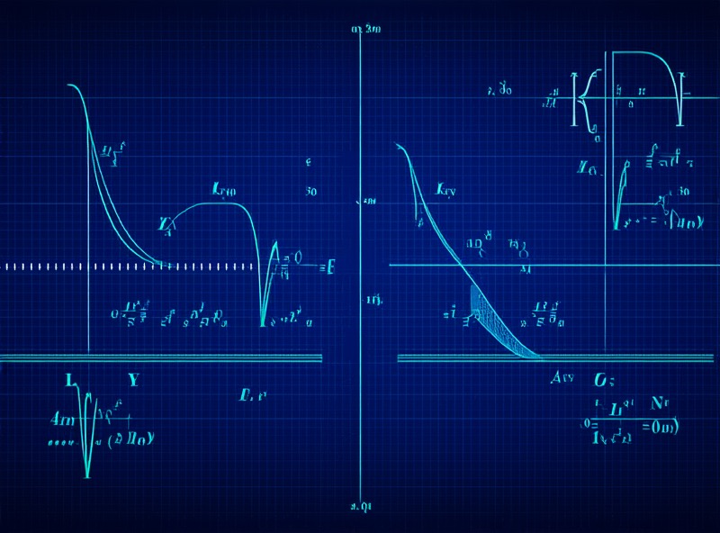
Laplace Transform Calculator
Calculate Laplace transforms and inverse transforms with step-by-step solutions. Explore transform pairs, properties, and applications to differential equations with interactive visualization.
View Simulation